Morning coffee: multilevel drift

20170204_185122

There is an abstract account of natural selection (Lewontin 1970) where one observes that any population of entities, whatever they may be, will evolve through natural selection if (1) there is variation, that (2) affects reproductive success, and (3) is heritable.

I don’t know how I missed this before, but it recently occurred to me that there must be a similarly abstract account of drift, where a population will evolve through drift if there is (1) variation, (2) that is heritable, and (3) sampling due to finite population size.

Drift may not be negligible, especially since at a higher level of organization, the population size should be smaller, making natural selection relatively less efficient.

@sweden recap

So, a couple of weeks ago I tweeted from the @sweden account. This is a short recap of some things that were said, and a few links that I promised people. Overall I think it went pretty well. I didn’t tweet as much as some other curators, but much much more than I usually do. This also meant I did spend my lunch and coffee breaks looking at my phone. My tweets are collected here, if for some reason you’d care to read them.

Of course, tweeting from a rotating curation account is very different from the way I normally use Twitter. First, I read much more than I write. One of the main purposes of Twitter, for me, is to get a steady stream of links to read. That doesn’t really work on an account that follows much more and entirely different people. A lot of what I wrote was prepared monologue, but I don’t think that’s necessarily a bad thing. I follow a lot of people on Twitter for their monologues. Also, thankfully, a lot of people asked me questions! Another thing that struck me is that so few people were unpleasant. There were a few extreme right folks who wanted me to retweet their racist tweets, but only a few. Then, a few felt the need to tell me that I’m utterly boring, which is fine. Someone lamented the fact that all curators are uneducated about the proper use of Twitter (it’s probably to build your personal brand or something). Also, a certain Swedish celebrity got put on ignore so I wouldn’t have to see him tagging each tweet with ”@sweden”. But that was pretty much all.

I talked quite a bit about my research. I spent more or less a full day on the chicken comb as a sexual ornament and genetics of comb mass. We discussed domestication as an evolutionary process, tonic immobility, and how to measure gene expression for eQTL mapping. I also wrote about Kauai feral chickens … And what I actually do in a day nowadays, that is: writing R code.

I got a question about what to say to your creationist friend. I think this depends on what the creationist friend believes and what their objections to evolution are. Unfortunately, I don’t think there is a simple knock-down argument against all forms of creationism, except that evolution works really well and has a lot of evidence going for it. I certainly don’t think it will do to rely on methodological naturalism and say that ”creation would be a supernatural event and outside the scope of science”. First, because I don’t think that is how science works. Say if unicorns, miraculous healing, and species popping into existence without relation to other species were actually part of the world, wouldn’t we want to study that? Second, that will never convince anyone, except of the irrelevance of science to their worldview.

But I think there are a handful of things that creationists often take issue with. First, some don’t believe in sequence variants creating new functions. This is often described with slogans about information, and how it cannot be created by random mutation. I don’t think ”sequence information” is a particularly useful concept, and would much prefer to talk about function and adaptation. That is what is important, after all, organisms acquiring new adaptations. It turns out, new functions arising can be observed, particularly in microorganisms. Some really fun and well-studied example occur in the Long Term Evolution Experiment; see Richard Lenski’s blog which has explanatory posts and links to papers.

Second, the formation of species come up a lot in these discussions. This is a bit tricky, because it’s not always clear what constitutes different species. The definition most people have heard is probably that individuals belong to different species if they cannot have fertile offspring. But just think of asexually reproducing organisms. There, individuals belong to different species if they’re sufficiently different. So we already have what is needed to understand the formation of species in the evolution of new functions. When it comes to sexually reproducing organisms, there are examples of the evolution of reproductive isolation — cases where it seems to be ongoing or to have happened recently. (See for instance this paper on hybrid incompatibility in Mimulus guttatus; I have blogged about it, but only in Swedish)

Third, there is the question of relatedness between species. In particular, some creationists really hate the idea that humans are apes. I think it is important to emphasize a couple of things that evolution does not say about humans and other apes. By the way, this isn’t just confusing for creationists, but for everyone. Evolution does not mean that humans descend from extant apes. Look at this phylogenetic tree from Perelman & al 2011. This is just like a family tree, but of populations: we see how chimps and humans have a recent common ancestor population. This is different than claiming that we would descend from extant chimps. Of course, chimps have also changed since the common ancestor, although not in the same ways as humans. (Again, I’ve written about this before in Swedish.)

journal.pgen.1001342.g001

Speaking of unicorns, I of course celebrated unicorn Friday:

Someone asked whether you can keep fruit flies for amateur genetics at home. That should be quite possible, and I don’t see any real problems with it either. The fruit fly community has really strong culture of classical genetics with crosses and stocks. I don’t know if stock centres would deliver to private customers, but I don’t see why they wouldn’t — except for transgenic flies. It turned out, however, that transgenic flies was actually what the person asking was after. And of course, I can’t recommend that. I must say, I have mixed feelings about do-it-yourself biotechnology. On the one hand, some home molecular biology should be possible and rewarding. On the other hand, a lot of things routinely used in molecular labs are actually really dangerous if misused, and not just for the user. For example, when making any type of construct in transgenic bacteria, antibiotics and antibiotic resistance genes are the standard screening markers. They are used to pick out the bacteria that have incorporated the piece of DNA you care about. This is not the kind of stuff you want to use without proper containment. So, in the fly example, you would not only have to handle the flies, but also transgenic antibiotic resistant bacteria safely and legally. Then again, a lot of the genetics I care about does not involve any of that, and could very well be done in a basement.

The @sweden account caught me under a teaching week; otherwise, all of my photos would’ve been my computer, my pen and my coffee mug. Now I got to walk the followers through agarose gel electrophoresis and a little transformation of bacteria:

And, finally, Swedish spring:

Finding the distance from ChIP signals to genes

I’ve had a couple of months off from blogging. Time for some computer-assisted biology! Robert Griffin asks on Stack Exchange about finding the distance between HP1 binding sites and genes in Drosophila melanogaster.  We can get a rough idea with some public chromatin immunoprecipitation data, R and the wonderful BEDTools.

Finding some binding sites

There are indeed some ChIP-seq datasets on HP1 available. I looked up these ones from modENCODE: modENCODE_3391 and modENCODE_3392, using two different antibodies for Hp1b in 16-24 h old embroys. I’m not sure since the modENCODE site doesn’t seem to link datasets to publications, but I think this is the paper where the results are reported: A cis-regulatory map of the Drosophila genome (Nègre & al 2011).

What they’ve done, in short, is cross-linking with formaldehyde, sonicate DNA into fragments, capture fragments with either of the two antibodies and sequence those fragments. They aligned reads with Eland (Illumina’s old proprietary aligner) and called peaks (i.e. regions where there is a lot of reads, which should reflect regions bound by Hp1b) with MACS. We can download their peaks in general feature format.

I don’t know whether there is any way to make completely computation predictions of Hp1 binding sites but I doubt it.

Some data cleaning

The files are available from ftp, and for the below analysis I’ve unzipped them and called them modENCODE_3391.gff3 and modENCODE_3392.gff3. GFF is one of all those tab separated text files that people use for genomic coordinates. If you do any bioinformatics type work you will have to convert back and forth between them and I suggest bookmarking the UCSC Genome Browser Format FAQ.

Even when we trust in their analysis, some processing of files is always required. In this case, MACS sometimes outputs peaks with negative start coordinates in the beginning of a chromosome. BEDTools will have none of that, because ”malformed GFF entry at line … Start was greater than end”. In this case, it happens only at a few lines, and I decided to set those start coordinates to 1 instead.

We need a small script to solve that. As I’ve written before, any language will do, but I like R and tend to do my utility scripting in R (and bash). If the files were incredibly huge and didn’t fit in memory, we’d have to work through the files line by line or chunk by chunk. But in this case we can just read everything at once and operate on it with vectorised R commands, and then write the table again.

modENCODE_3391 <- read.table("modENCODE_3391.gff3", stringsAsFactors=F, sep="\t")
modENCODE_3392 <- read.table("modENCODE_3392.gff3", stringsAsFactors=F, sep="\t")

fix.coord <- function(gff) {
  gff$V4[which(gff$V4 < 1)] <- 1
  gff
}

write.gff <- function(gff, file) {
  write.table(gff, file=file, row.names=F, col.names=F,
              quote=F, sep="\t")
}

write.gff(fix.coord(modENCODE_3391), file="cleaned_3391.gff3")
write.gff(fix.coord(modENCODE_3392), file="cleaned_3392.gff3")

Flybase transcripts

To find the distance to genes, we need to know where the genes are. The best source is probably the annotation made by Flybase, which I downloaded from the Ensembl ftp in General transfer format (GTF, which is close enough to GFF that we don’t have to care about the differences right now).

This file contains a lot of different features. We extract the transcripts and find where the transcript model starts, taking into account whether the transcript is in the forward or reverse direction (this information is stored in columns 4, 5 and 7 of the GTF file). We store this in a new GTF file of transcript start positions, which is the one we will feed to BEDTools:

ensembl <- read.table("Drosophila_melanogaster.BDGP5.75.gtf",
                      stringsAsFactors=F, sep="\t")

transcript <- subset(ensembl, V3=="transcript")
transcript.start <- transcript
transcript.start$V3 <- "transcript_start"
transcript.start$V4 <- transcript.start$V5 <- ifelse(transcript.start$V7 == "+",
                                                     transcript$V4, transcript$V5)

write.gff(transcript.start, file="ensembl_transcript_start.gtf")

Finding distance with BEDTools

Time to find the closest feature to each transcript start! You could do this in R with GenomicRanges, but I like BEDTools. It’s a command line tool, and if you haven’t already you will need to download and compile it, which I recall being painless.

bedtools closest is the command that finds, for each feature in one file, the closest feature in the other file. The -a and -b flags tells BEDTools which files to operate on, and the -d flag that we also want it to output the distance. BEDTools writes output to standard out, so we use ”>” to capture it in a text file.

Here is the bash script. I put the above R code in clean_files.R and added it as an Rscript line at the beginning, so I could run it all with one file.

#!/bin/bash
Rscript clean_files.R

bedtools closest -d -a ensembl_transcript_start.gtf -b cleaned_3391.gff3 \
    > closest_element_3391.txt
bedtools closest -d -a ensembl_transcript_start.gtf -b cleaned_3392.gff3 \
    > closest_element_3392.txt

Some results

With the resulting file we can go back to R and ggplot2 and draw cute graphs like this, which shows the distribution of distances from transcript to Hp1b peak for protein coding and noncoding transcripts separately. Note the different y-scales (there are way more protein coding genes in the annotation) and the 10-logarithm plus one transformation on the x-axis. The plus one is to show the zeroes; BEDTools returns a distance of 0 for transcripts that overlap a Hp1b site.

closest_3391 <- read.table("~/blogg/dmel_hp1/closest_element_3391.txt", header=F, sep="\t")

library(ggplot2)
qplot(x=log10(V19 + 1), data=subset(closest_3391, V2 %in% c("protein_coding", "ncRNA"))) +
  facet_wrap(~V2, scale="free_y")

distance_hist

Or by merging the datasets from different antibodies, we can draw this strange beauty, which pretty much tells us that the antibodies do not give the same result in terms of the closest feature. To figure out how they differ, one would have to look more closely into the genomic distribution of the peaks.

closest_3392 <- read.table("~/blogg/dmel_hp1/closest_element_3392.txt", header=F, sep="\t")

combined <- merge(closest_3391, closest_3392,
                  by.x=c("V1", "V2","V4", "V5", "V9"),
                  by.y=c("V1", "V2","V4", "V5", "V9"))

qplot(x=log10(V19.x+1), y=log10(V19.y+1), data=combined)

between_antibodies

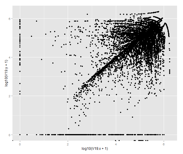
(If you’re wondering about the points that end up below 0, those are transcripts where there are no peaks called on that chromosome in one of the datasets. BEDTools returns -1 for those that lack matching features on the same chromosome and R will helpfully transform them to -Inf.)

About the DGRP

The question mentioned the DGRP. I don’t know that anyone has looked at ChIP in the DGRP lines, but wouldn’t that be fun? Quantitative genetics of DNA binding protein variation in DGRP and integration with eQTL … What one could do already, though, is take the interesting sites of Hp1 binding and overlap them with the genetic variants of the DGRP lines. I don’t know if that would tell you much — does anyone know what kind of variant would affect Hp1 binding?

Happy hacking!

Morning coffee: the selfish gene versus the world

kaffe_knä

The distinction between ”gene” in the sense of an allele at some locus and ”gene” in the sense of a dna sequence with a name and some function seems easy enough, but still causes a lot of confusion, both in popular and scientific literature.

This was very clear a few months ago when science journalist David Dobbs published his ”Die selfish gene, die” and a few weeks of debate broke out. In my opinion it’s not a particularly good piece, but I agree with Dobbs that the ”selfish gene” metaphor sometimes invites misunderstandings. The article itself displays a few of them, when it suggests that evolution and genetics as understood before the age of microarrays are somehow at odds with the importance of gene regulation or phenotypic plasticity. I suspect that many of these problems stem from the double meaning of the word gene. Other examples are found in headlines claiming that researchers have found the gene for something or the confusion about the word pleiotropy (Paaby & Rockman 2012).

When Dawkins wrote about the selfish gene, he did not mean the selfish dna sequence encoding a protein; he meant the selfish genetic variant causing differences in fitness between individuals. (Or rather, a set of genetic variants in sufficiently close linkage to seldom be separated by recombination.) The book is not about molecular genes. As anyone who actually read it knows, it deals mostly with behaviour using game theory approaches. This does not mean that Dawkins denied that there are actual molecular genes doing the mechanistic work, but that he analysed the situation mostly on a different level. And had he chosen to write only about known sequence variants with adaptive effects on behaviour it would have been a very short book.

Of course the word ”selfish”, while I agree that it is the proper word in the sense that Dawkins intended, is great for those who want to point to instances where people are horrible to each other and tell you that it’s all because of evolution. But I think that is a bigger issue that will not be solved by tweaking popular science metaphors. By the way, that is completely contrary to Dawkins’ intentions, which were to popularise the evolutionary models that explain why animals are not always horrible to each other, even though their behaviour is shaped by natural selection.

Journal club of one: ”Functionally enigmatic genes: a case study of the brain ignorome”

This recent paper, Pandey & al (2014), made me interested because I’m in the business of finding genes for traits, and have spent quite some time looking at lists of gene names and annotation database output. One is tempted to look for the ”outstanding candidates” that ”make biological sense” (quotes intended as scare quotes), but the truth is probably that no-one knows what genes and functions we should expect to be affected by genetic variation in, for instance, behaviour. This paper tries to make the case for the unknown parts of the brain transcriptome; they use data about gene expression, protein domains, paralogs and literature to argue that the unknown genes are unknown for no good reason and that they might be just as important as genes that happen to be well-known.

They found genes that are had a high ratio of expression in brain to average expression in other tissues of C57BL/6J and DBA/2J mice and searched PubMed for these genes in combination with neuroscience-related keywords. Some of them have few citations and these are their selectively expressed but little studied genes. They then make a series of comparisons between these and well-studied genes. It turns out the only major difference is that well-studied genes were discovered (entered into GenBank) earlier.

Comments:

I don’t know to what extent these results are suprising. I was not surprised by their main conclusion, but then again, that maybe my opinion was mostly prejudice. There is a literature on biases in the functional genomics literature, but I don’t know much about it. And apparently neither did the authors, initially, as Robert Williams writes in a comment on the PLOS ONE website:

We did not rediscover the lovely work of Robert Hoffmann (now head of WikiGene) until the paper had been submitted in succession to six higher profile journals … Hoffmann and colleagues showed that social factors account for much of the annotation imbalance for genes.

I love the idea of authors writing an informal comment about the background of the paper like this.

The coexpression network results show some of the little known genes are just as connected as known important genes. This suggest some of the unknown genes might be important too, if we can trust that coexpression hub genes are likely to be important (for various values of ”important”). Maybe this is a scientific opportunity for some neuroscientist. Several people I’ve talked with has imagined future Big Science initiatives to describe the function of unknown genes — ”divide them up between labs and characterise them!” — and some initiatives exist, such as the IMPC. On the other hand, how do we know that we really find the most important and interesting functions of a gene? The skeptic in me thinks that going bottom up, from gene to phenotype, will miss the most interesting surprising phenotypes.

I think ”ignorome” is one of those unnecessary bad omics words, which is why I’ve avoided using it.

Their PubMed query was restricted to mouse, human and rat. I wonder why. Maybe there could be something useful from fruit flies or roundworms?

Overall, a fun paper that I recommend reading over a few cups of coffee!

Literature

Pandey AK, Lu L, Wang X, Homayouni R, Williams RW (2014) Functionally Enigmatic Genes: A Case Study of the Brain Ignorome. PLoS ONE 9(2): e88889. doi:10.1371/journal.pone.0088889

From my halftime seminar

A couple of weeks ago I presented my halftime seminar at IFM Biology, Linköping university. The halftime at our department isn’t a particularly dramatic event, but it means that after you’ve been going for two and a half years (since a typical Swedish PhD programme is four years plus 20% teaching to a total of five years), you get to talk about what you’ve been up to and discuss it with an invited opponent. I talked about combining genetic mapping and gene expression to search for quantitative trait genes for chicken domestication traits, and the work done so far particularly with relative comb mass. To give my esteemed readers an overview of what my project is about, here come a few of my slides about the mapping work — it is described in detail in Johnsson & al (2012). Yes, it does feel very good to write that — shout-outs to all the coauthors! This is part what I said on the seminar, part digression more suited for the blog format. Enjoy!

Slide04(Photo: Dominic Wright)

The common theme of my PhD project is genetic mapping and genetical genomics in an experimental intercross of wild and domestic chickens. The photo shows some of them as chicks. Since plumage colour is one of the things that segregate in this cross, their feathers actually make a very nice illustration of what is going on. We’re interested in traits that differ between wild and domestic chickens, so we use a cross based on a Red Jungefowl male and three domestic White Leghorn females. Their offspring have been mated with each other for several generations, giving rise to what is called an advanced intercross line. Genetic variants that cause differences between White Leghorn and Red Jungefowl chickens will segregate among the birds of the cross, and are mixed by recombination at meiosis. Some of the birds have the Red Junglefowl variant and some have the White Leghorn variant at a given part of their genome. By measuring traits that vary in the cross, and genotyping the birds for a map of genetic markers, we can find chromosomal chunks that are associated with particular traits, i.e. regions of the genome where we’re reasonably confident harbour a variant affecting the trait. These chromosomal chunks tend to be rather large, though, and contain several genes. My job is to use gene expression measurements from the cross to help zero in on the right genes.

The post continues below the fold! Fortsätt läsa