Using R: plyr to purrr, part 1

This is the second post about my journey towards writing more modern Tidyverse-style R code; here is the previous one. We will look at the common case of taking subset of data out of a data frame, making some complex R object from them, and then extracting summaries from those objects.

More nostalgia about plyr

I miss the plyr package. Especially ddply, ldply, and dlply, my favourite trio of R functions of all times. Yes, the contemporary Tidyverse package dplyr is fast and neat. And those plyr functions operating on arrays were maybe overkill; I seldom used them. But plyr was so smooth, so beautiful, and — after you’ve bashed your head against it for some time and it changed your mind — so intuitive. The package still exists, but it’s retired, and we shouldn’t keep writing R code like it’s 2009, should we?

I used to like to do something like this: take a data frame, push it through a function that returns some complex object, store those objects in a list, and then map various functions over that list to extract the parts I care about. What is the equivalent in the new idiom? To do the same thing but with the purrr package, of course! purrr replaces the list-centric parts of plyr, while dplyr covers data frame-centric summarisation, mutation and so on.

For this example we will be using the lm function on subsets of data and store the model object. It’s the simple case that everyone reaches for to demonstrate these features, but it’s a bit dubious. If you find yourself fitting a lot of linear models to subsets, maybe there are other models you should think about Especially here, when the fake data just happens to come from a multilevel model with varying intercepts … But in this case, let’s simulate a simple linear regression and look at the coefficients we get out.

set.seed(20210807)

n_groups <- 10
group_sizes <- rpois(n_groups, 10)
n <- sum(group_sizes)

fake_data <- tibble(id = 1:n,
                    group = rep(1:n_groups,
                                times = group_sizes),
                    predictor = runif(n, 0, 1))
group_intercept <- rnorm(n_groups, 0, 1)

fake_data$response <- fake_data$predictor * 10 +
  group_intercept[fake_data$group] +
  rnorm(n)

And here is the plyr code: First, dlply takes us from a data frame, splitting it by group, to a list of linear models. Then, ldply takes us from the list of models to a data frame of coefficients. tidy is a function from the wonderful broom package which extracts the same information as you would get in the rather unwieldy object from summary(lm), but as a data frame.

library(plyr)
library(broom)

fit_model <- function(data) {
  lm(response ~ predictor, data)
}

models <- dlply(fake_data,
                     "group",
                     fit_model)
result <- ldply(models, tidy)

This is what the results might looks like. Notice how ldply adds the split labels nicely into the group column, so we know which rows came from which subset.

   group        term   estimate std.error  statistic      p.value
1      1 (Intercept) -0.2519167 0.5757214 -0.4375670 6.732729e-01
2      1   predictor 10.6136902 1.0051490 10.5593207 5.645878e-06
3      2 (Intercept)  3.1528489 0.6365294  4.9531864 7.878498e-04
4      2   predictor  8.2075766 1.1458702  7.1627452 5.292586e-05
5      3 (Intercept) -0.8103777 0.6901212 -1.1742542 2.786901e-01
...

split/map: The modern synthesis

If we pull out purrr, we can get the exact same table like so. The one difference is that we get a tibble (that is, a contemporary, more well-behaved data frame) out of it instead of a base R data.frame.

library(purrr)

models <- map(split(fake_data,
                    fake_data$group),
                    fit_model)
result <- map_df(models,
                 tidy,
                 .id = "group")
# A tibble: 80 x 6
   group term        estimate std.error statistic  p.value
                            
 1 1     (Intercept)     1.67     0.773      2.16 6.32e- 2
 2 1     predictor       8.67     1.36       6.39 2.12e- 4
 3 2     (Intercept)     4.11     0.566      7.26 4.75e- 5
 4 2     predictor       8.19     1.11       7.36 4.30e- 5
 5 3     (Intercept)    -7.50     0.952     -7.89 9.99e- 5
 6 3     predictor      11.5      1.75       6.60 3.03e- 4
 7 4     (Intercept)   -19.8      0.540    -36.7  7.32e-13
 8 4     predictor      11.5      0.896     12.8  5.90e- 8
 9 5     (Intercept)   -12.4      1.03     -12.0  7.51e- 7
10 5     predictor       9.69     1.82       5.34 4.71e- 4
# … with 70 more rows

First, the base function split lets us break the data into subsets based on the values of a variable, which in this case is our group variable. The output of this function is a list of data frames, one for each group.

Second, we use map to apply a function to each element of that list. The function is the same modelling function that we used above, which shoves the data into lm. We now have our list of linear models.

Third, we apply the tidy function to each element of that list of models. Because we want the result to be one single data frame consolidating the output from each element, we use map_df, which will combine the results for us. (If we’d just use map again, we would get a list of data frames.) The .id argument tells map to add the group column that indicates what element of the list of models each row comes from. We want this to be able to identify the coefficients.

If we want to be fancy, we can express with the Tidyverse-related pipe and dot notation:

library(magrittr)

result <- fake_data %>%
  split(.$group) %>%
  map(fit_model) %>%
  map_df(tidy, .id = "group")

Nesting data into list columns

This (minus the pipes) is where I am at in most of my R code nowadays: split with split, apply with map and combine with map_dfr. This works well and looks neater than the lapply/Reduce solution discussed in part 0.

We can push it a step further, though. Why take the linear model out of the data frame, away from its group labels any potential group-level covariates — isn’t that just inviting some kind of mix-up of the elements? With list columns, we could store the groups in a data frame, keeping the data subsets and any R objects we generate from them together. (See Wickham’s & Grolemund’s R for Data Science for a deeper case study of this idea.)

library(dplyr)
library(tidyr)

fake_data_nested <- nest(group_by(fake_data, group),
                         data = c(id, predictor, response))

fake_data_models <- mutate(fake_data_nested,
                           model = map(data,
                                       fit_model),
                           estimates = map(model,
                                           tidy))

result <- unnest(fake_data_models, estimates)

First, we use the nest function to create a data frame where each row is a group, and the ”data” column contains the data for that subset.

Then, we add two list columns to that data frame: our list of models, and then our list of data frames with the coefficients.

Finally, we extract the estimates into a new data frame with unnest. The result is the same data frame of coefficients and statistics, also carrying along the data subsets, linear models and coefficents.

The same code with pipes:

fake_data %>% 
  group_by(group) %>% 
  nest(data = c(id, predictor, response)) %>% 
  mutate(model = map(data, fit_model),
         estimates = map(model, tidy)) %>% 
  unnest(estimates) -> ## right way assignment just for kicks
  result

I’m still a list column sceptic, but I have to concede that this is pretty elegant. It gets the job done, it keeps objects that belong together together so that there is no risk of messing up the order, and it is not that much more verbose. I especially like that we can run the models and extract the coefficients in the same mutate call.

Coda: mixed model

Finally, I can’t resist comparing the separate linear models to a linear mixed model of all the data.

We use lme4 to fit a varying-intercept model, a model that puts the same coefficient on the slope between the response and predictor in each group, but allows the intercepts to vary between groups, assuming them to be drawn from the same normal distribution. We put the coefficients from the linear models fit in each group separately and the linear mixed model together in the same data frame to be able to plot them.

library(ggplot2)
library(lme4)

model <- lmer(response ~ (1|group) + predictor,
              fake_data)

lm_coef <- pivot_wider(result,
                       names_from = term,
                       values_from = estimate,
                       id_cols = group)

lmm_coef <- cbind(group = levels(model@flist$group),
                  coef(model)$group)

model_coef <- rbind(transform(lm_coef, model = "lm"),
                    transform(lmm_coef, model = "lmm"))

colnames(model_coef)[2] <- "intercept"

ggplot() +
  geom_point(aes(x = predictor,
                 y = response,
                 colour = factor(group)),
             data = fake_data) +
  geom_abline(aes(slope = predictor,
                  intercept = intercept,
                  colour = factor(group),
                  linetype = model),
              data = model_coef) +
  theme_bw() +
  theme(panel.grid = element_blank())

As advertised, the linear mixed model has the same slope in every group, and intercepts pulled closer to the mean. Now, we know that this is a good model for these fake data because we created them, and in the real world, that is obviously not the case … The point is: if we are going to fit a more complex model of the whole data, we want to be able to explore alternatives and plot them together with the data. Having elegant ways to transform data frames and summarise models at our disposal makes that process smoother.

Using R: setting a colour scheme in ggplot2

Note to self: How to quickly set a colour scheme in ggplot2.

Imagine we have a series of plots that all need a uniform colour scale. The same category needs to have the same colour in all graphics, made possibly with different packages and by different people. Instead of hard-coding the colours and the order of categories, we can put them in a file, like so:

library(readr)
colours <- read_csv("scale_colours.csv")
# A tibble: 5 x 2
  name   colour 
      
1 blue   #d4b9da
2 red    #c994c7
3 purple #df65b0
4 green  #dd1c77
5 orange #980043

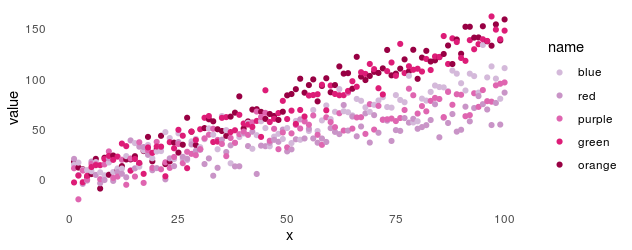
Now a plot with default colours, using some made-up data:

x <- 1:100

beta <- rnorm(5, 1, 0.5)

stroop <- data.frame(x,
                     sapply(beta, function(b) x * b + rnorm(100, 1, 10)))
colnames(stroop)[2:6] <- c("orange", "blue", "red", "purple", "green") 

data_long <- pivot_longer(stroop, -x)

plot_y <- qplot(x = x,
                y = value,
                colour = name,
                data = data_long) +
  theme_minimal() +
  theme(panel.grid = element_blank())

Now we can add the custom scale like this:

plot_y_colours <- plot_y + 
  scale_colour_manual(limits = colours$name,
                      values = colours$colour)


Using R: From gather to pivot

Since version 1.0.0, released in September, the tidyr package has a new replacement for the gather/spread pair of functions, called pivot_longer/pivot_wider. (See the blog post about the release. It can do a lot of cool things.) Just what we needed, another pair of names for melt/cast, right?

Yes, I feel like this might just be what we need!

My journey started with reshape2, and after a bit of confusion, I internalised the logic of melt/cast. Look at this beauty:

library(reshape2)
fake_data <- data.frame(id = 1:20,
                        variable1 = runif(20, 0, 1),
                        variable2 = rnorm(20))
melted <- melt(fake_data, id.vars = "id")

This turns a data frame that looks like this …

  id  variable1   variable2
1  1 0.10287737 -0.21740708
2  2 0.04219212  1.36050438
3  3 0.78119150  0.09808656
4  4 0.44304613  0.48306900
5  5 0.30720140 -0.45028374
6  6 0.42387957  1.16875579

… into a data frame that looks like this:

  id  variable      value
1  1 variable1 0.10287737
2  2 variable1 0.04219212
3  3 variable1 0.78119150
4  4 variable1 0.44304613
5  5 variable1 0.30720140
6  6 variable1 0.42387957

This is extremely useful. Among other things it comes up all the time when using ggplot2.

Then, as I detailed in a post two years ago, I switched to tidyr as that became the replacement package. ”Gather” and ”spread” made no sense to me as descriptions of operations on a data frame. To be fair, ”melt” and ”cast” felt equally arbitrary, but by that time I was used to them. Getting the logic of the arguments, the order, what needed quotation marks and not, took some staring at examples and a fair bit of trial and error.

Here are some examples. If you’re not used to these functions, just skip ahead, because you will want to learn the pivot functions instead!

library(tidyr)
melted <- gather(fake_data, variable, value, 2:3)
 
## Column names instead of indices
melted <- gather(fake_data, variable, value, variable1, variable2)
 
## Excluding instead of including
melted <- gather(fake_data, variable, value, -1)
 
## Excluding using column name
melted <- gather(fake_data, variable, value, -id)

Enter the pivot functions. Now, I have never used pivot tables in any spreadsheet software, and in fact, the best way to explain them to me was to tell me that they were like melt/cast (and summarise) … But pivot_longer/pivot_wider are friendlier on first use than gather/spread. The naming of both the functions themselves and their arguments feel like a definite improvement.

long <- pivot_longer(fake_data, 2:3,
                     names_to = "variable",
                     values_to = "value")
# A tibble: 40 x 3
      id variable    value
           
 1     1 variable1  0.103 
 2     1 variable2 -0.217 
 3     2 variable1  0.0422
 4     2 variable2  1.36  
 5     3 variable1  0.781 
 6     3 variable2  0.0981
 7     4 variable1  0.443 
 8     4 variable2  0.483 
 9     5 variable1  0.307 
10     5 variable2 -0.450 
# … with 30 more rows

We tell it into what column we want the names to go, and into what column we want the values to go. The function is named after a verb that is associated with moving things about in tables all the way to matrix algebra, followed by an adjective (in my opinion the most descriptive, out of the alternatives) that describes the layout of the data that we want.

Or, to switch us back again:

wide <- pivot_wider(long,
                    names_from = "variable",
                    values_from = "value")
# A tibble: 20 x 3
      id variable1 variable2
             
 1     1    0.103    -0.217 
 2     2    0.0422    1.36  
 3     3    0.781     0.0981
 4     4    0.443     0.483 
 5     5    0.307    -0.450 
 6     6    0.424     1.17  

Here, instead, we tell it where we want the new column names taken from and where we want the new values taken from. None of this is self-explanatory, by any means, but they are thoughtful choices that make a lot of sense.

We’ll see what I think after trying to explain them to beginners a few times, and after I’ve fought warning messages involving list columns for some time, but so far: well done, tidyr developers!

Using R: Correlation heatmap with ggplot2

(This post was originally written on 2013-03-23. Since then, it has persistently remained one of my most visited posts, and I’ve decided to revisit and update it. I may do the same to some other old R-related posts that people still arrive on through search engines. There was also this follow-up, which I’ve now incorporated here.)

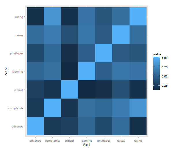
Just a short post to celebrate when I learned how incredibly easy it is to make a heatmap of correlations with ggplot2 (with some appropriate data preparation, of course). Here is a minimal example using the reshape2 package for preparation and the built-in attitude dataset:

library(ggplot2)
library(reshape2)
qplot(x = Var1, y = Var2,
      data = melt(cor(attitude)),
      fill = value,
      geom = "tile")

attitude_heatmap

What is going on in that short passage?

  • cor makes a correlation matrix with all the pairwise correlations between variables (twice; plus a diagonal of ones).
  • melt takes the matrix and creates a data frame in long form, each row consisting of id variables Var1 and Var2 and a single value.
  • We then plot with the tile geometry, mapping the indicator variables to rows and columns, and value (i.e. correlations) to the fill colour.

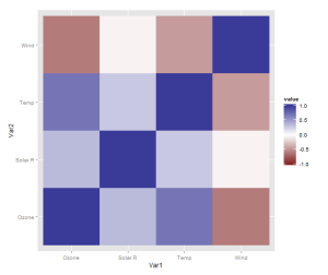
However, there is one more thing that is really need, even if just for the first quick plot one makes for oneself: a better scale. The default scale is not the best for correlations, which range from -1 to 1, because it’s hard to tell where zero is. Let’s use the airquality dataset for illustration as it actually has some negative correlations. In ggplot2, a scale that has a midpoint and a different colour in each direction is called scale_colour_gradient2, and we just need to add it. I also set the limits to -1 and 1, which doesn’t change the colour but fills out the legend for completeness. Done!

data <- airquality[,1:4]
qplot(x = Var1, y = Var2,
      data = melt(cor(data, use = "p")),
      fill = value,
      geom = "tile") +
   scale_fill_gradient2(limits = c(-1, 1))

correlation_heatmap2

Finally, if you’re anything like me, you may be phasing out reshape2 in favour of tidyr. If so, you’ll need another function call to turn the matrix into a data frame, like so:

library(tidyr)

correlations <- data.frame(cor(data, use = "p"))
correlations$Var1 <- rownames(correlations)
melted <- gather(correlations, "value", "Var2", -Var1)

qplot(x = Var1, y = Var2,
      data = melted,
      fill = value,
      geom = "tile") +
   scale_fill_gradient2(limits = c(-1, 1))

The data preparation is no longer a oneliner, but, honestly, it probably shouldn’t be.

Okay, you won’t stop reading until we’ve made a solution with pipes? Sure, we can do that! It will be pretty gratuitous and messy, though. From the top!

library(magrittr)

airquality %>%
    '['(1:4) %>%
    data.frame %>%
    transform(Var1 = rownames(.)) %>%
    gather("Var2", "value", -Var1) %>%
    ggplot() +
        geom_tile(aes(x = Var1,
                      y = Var2,
                      fill = value)) +
        scale_fill_gradient2(limits = c(-1, 1))

Using R: reshape2 to tidyr

Tidy data — it’s one of those terms that tend to confuse people, and certainly confused me. It’s Codd’s third normal form, but you can’t go around telling that to people and expect to be understood. One form is ”long”, the other is ”wide”. One form is ”melted”, another ”cast”. One form is ”gathered”, the other ”spread”. To make matters worse, I often botch the explanation and mix up at least two of the terms.

The word is also associated with the tidyverse suite of R packages in a somewhat loose way. But you don’t need to write in a tidyverse-style (including the %>%s and all) to enjoy tidy data.

But Hadley Wickham’s definition is straightforward:

In tidy data:
1. Each variable forms a column.
2. Each observation forms a row.
3. Each type of observational unit forms a table.

In practice, I don’t think people always take their data frames all the way to tidy. For example, to make a scatterplot, it is convenient to keep a couple of variables as different columns. The key is that we need to move between different forms rapidly (brain time-rapidly, more than computer time-rapidly, I might add).

And not everything should be organized this way. If you’re a geneticist, genotypes are notoriously inconvenient in normalized form. Better keep that individual by marker matrix.

The first serious piece of R code I wrote for someone else was a function to turn data into long form for plotting. I suspect plotting is often the gateway to tidy data. The function was like what you’d expect from R code written by a beginner who comes from C-style languages: It reinvented the wheel, and I bet it had nested for loops, a bunch of hard bracket indices, and so on. Then I discovered reshape2.

library(reshape2)
fake_data <- data.frame(id = 1:20,
                        variable1 = runif(20, 0, 1),
                        variable2 = rnorm(20))
melted <- melt(fake_data, id.vars = "id")

The id.vars argument is to tell the function that the id column is the key, a column that tells us which individual each observation comes from. As the name suggests, id.vars can name multiple columns in a vector.

So the is the data before:

  id   variable1    variable2
1  1 0.938173781  0.852098580
2  2 0.408216233  0.261269134
3  3 0.341325188  1.796235963
4  4 0.958889279 -0.356218000

And this is after. We go from 20 rows to 40: two variables times 20 individuals.

  id  variable       value
1  1 variable1 0.938173781
2  2 variable1 0.408216233
3  3 variable1 0.341325188
4  4 variable1 0.958889279

And now: tidyr. tidyr is the new tidyverse package for rearranging data like this.

The tidyr equivalent of the melt function is called gather. There are two important differences that messed with my mind at first.

The melt and gather functions take the opposite default assumption about what columns should be treated as keys and what columns should be treated as containing values. In melt, as we saw above, we need to list the keys to keep them with each observation. In gather, we need to list the value columns, and the rest will be treated as keys.

Also, the second and third arguments (and they would be the first and second if you piped something into it), are the variable names that will be used in the long form data. In this case, to get a data frame that looks exactly the same as the first, we will stick with ”variable” and ”value”.

Here are five different ways to get the same long form data frame as above:

library(tidyr)
melted <- gather(fake_data, variable, value, 2:3)

## Column names instead of indices
melted <- gather(fake_data, variable, value, variable1, variable2)

## Excluding instead of including
melted <- gather(fake_data, variable, value, -1)

## Excluding using column name
melted <- gather(fake_data, variable, value, -id)

## With pipe
melted <- fake_data %>% gather(variable, value, -id)

Usually, this is the transformation we need: wide to long. If we need to go the other way, we can use plyr’s cast functions, and tidyr’s gather. This code recovers the original data frame:

## plyr
dcast(melted, id ~  variable)

## tidyr
spread(melted, variable, value)