From my halftime seminar

A couple of weeks ago I presented my halftime seminar at IFM Biology, Linköping university. The halftime at our department isn’t a particularly dramatic event, but it means that after you’ve been going for two and a half years (since a typical Swedish PhD programme is four years plus 20% teaching to a total of five years), you get to talk about what you’ve been up to and discuss it with an invited opponent. I talked about combining genetic mapping and gene expression to search for quantitative trait genes for chicken domestication traits, and the work done so far particularly with relative comb mass. To give my esteemed readers an overview of what my project is about, here come a few of my slides about the mapping work — it is described in detail in Johnsson & al (2012). Yes, it does feel very good to write that — shout-outs to all the coauthors! This is part what I said on the seminar, part digression more suited for the blog format. Enjoy!

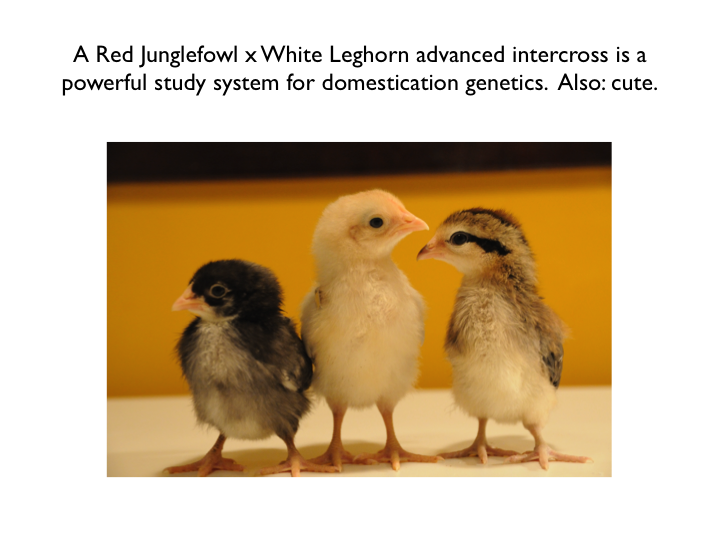(Photo: Dominic Wright)

The common theme of my PhD project is genetic mapping and genetical genomics in an experimental intercross of wild and domestic chickens. The photo shows some of them as chicks. Since plumage colour is one of the things that segregate in this cross, their feathers actually make a very nice illustration of what is going on. We’re interested in traits that differ between wild and domestic chickens, so we use a cross based on a Red Jungefowl male and three domestic White Leghorn females. Their offspring have been mated with each other for several generations, giving rise to what is called an advanced intercross line. Genetic variants that cause differences between White Leghorn and Red Jungefowl chickens will segregate among the birds of the cross, and are mixed by recombination at meiosis. Some of the birds have the Red Junglefowl variant and some have the White Leghorn variant at a given part of their genome. By measuring traits that vary in the cross, and genotyping the birds for a map of genetic markers, we can find chromosomal chunks that are associated with particular traits, i.e. regions of the genome where we’re reasonably confident harbour a variant affecting the trait. These chromosomal chunks tend to be rather large, though, and contain several genes. My job is to use gene expression measurements from the cross to help zero in on the right genes.

The post continues below the fold!

Several forces are in play in the domestication process. Imagine that these colourful circles are two alleles at a locus. Some of the variants of the wild population will be fixed by drift, and some relatively few of them will rise to prominence because they confer a selective advantage for life with humans, and the occasional new mutation will arise. Selection pressures probably also varied over the last 10 000 years, particularly the very strong artificial selection of modern chicken breeding.

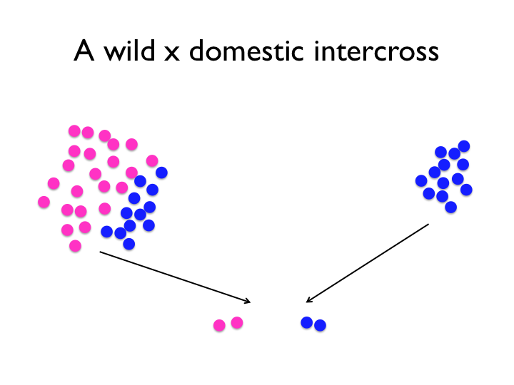
The experimental intercross compares and contrasts snapshots of a wild and domestic population. Note, however, that particularly for the wild population, one intercross will likely not capture all the relevant variation, and that the intercross experiment contains no information about the population allele frequencies. Of course, it is not as simple as the image might suggest — first, the wild population used is not really the same as the one chickens were domesticated from. Though, we rely on the fact that the Red Junglefowl hasn’t been through as dramatic a change as the rapid evolution that is domestication. Secondly, we can only detect variants that differ between the founders of the cross. If domestication variants exist at low frequencies in the wild population, then it’s increasingly likely that the founding rooster lacked those alleles. An experimental intercross means taking a genome from the domesticated pool and one from the non-domesticated pool and contrasting them.

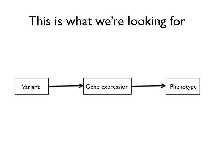
The targets of the experiment are genetic variants that work like the mechanism above. After reading some Lindley Darden, I became quite fond of this type of cartoon. Think of the above (which looks a lot like the directed acyclic graphs used for structural equations models and Bayesian networks, doesn’t it? It’s not a coincidence) is a mechanism sketch for a system that we’re searching for. From this part of the experiment, structural changes to protein coding genes are excluded by design, though we’re not entirely helpless when it comes to them either. The genetic mapping and genetical genomics experiment is set up to detect variants that act by means of changes in gene expression to influence certain domestication traits.

This slide shows the experiments mapped to the mechanism sketch. We type the birds of the intercross for a set of genetic markers and measure a bunch of organismal and molecular phenotypes.

Now is a good time to introduce a few slightly awkward terms that are sometimes used in the genetic mapping business. The mapping of quantitative traits, that is any trait that varies approximately as a continuous distribution, is called QTL mapping: Quantitative Trait Locus mapping. QTG and QTN refer to quantitative trait loci that have been resolved to a causal gene — Quantitative Trait Gene — and eventually a sequence variant — Quantitative Trait Nucleotide(s). I will try to avoid these acronyms below, but they’re sometimes used as shorthand.

Here’s another pice of jargon: eQTL. These smaller sketches show the genetic mapping steps of the experiment. Genetic mapping of the organismal trait establishes that there is a, so for unknown, genetic variant affecting it. It identifies the first component of the above mechanism. Genetic mapping of gene expression establishes the second part, that is, that there is some unknown genetic variant affecting an expression trait. If they are the same and the change in gene expression is mediating the change in the trait, we have a quantitative trait gene. eQTL mapping is just a fancy word for genetic mapping of an expression trait.

Now on to relative comb mass. The chicken comb is a pretty well-studied example of a sexual ornament that appears to signal mate quality in some way both for female and male chickens. Of course we’re curious to see if we can isolate a few of the genes and see what they do. Domestic chickens have bigger combs, relative to their body size, than Red Junglefowl, and the variation segregates in the intercrosses. We can use this fact to our advantage to map relative comb mass.

We’ve looked at the relative comb mass in three crosses, and the architecture looks similar. The above plot shows the known part of the chicken genome on the x-axis and the result of three mapping experiments as the black boxes. Each box represents the support interval for that QTL, that is, the region where we’re reasonably confident that there is a genetic variant affecting comb size. Wider boxes of course represent bigger uncertainty, and we immediately see that the F8-L13 experiment has the smallest boxes. That is the advanced intercross, generation eight. Intercrossing adds recombination events, so the 8th generation chickens have more mixed-up genomes, and give finer map resolution. F2-L13 is the second generation of the same intercross and F2-OS is the second generation of a different Red Jungefowl x White Leghorn cross, using the so called Obese Strain White Leghorn chickens. There are six regions of overlap where there is either shared variants, shared perturbed genes or at least clusters of perturbed genes between the crosses — all of which would be interesting.

The QTL with the largest effect size in the Red Junglefowl x L13 White Leghorn cross, both in the second and 8th generation, is located on chromsome 3. With the high mapping resolution of the advanced intercross, the interval is only 400 kb long and is located between two genes: HAO1 and BMP2. The first encodes an enzyme, hydroxoacid oxidase 1, that oxidises certain organic acids in the peroxisome; the second encods bone morphogenetic protein 2, which has multiple roles in development, including regulation of bone and cartilage development. The region in between them also contains a region of low heterozygosity found in the resequencing based study of Rubin & co; that’s the pink thing in the above figure. Low heterozygosity in the domestic populations means that (maybe) something in this region has been selected during chicken domestication. So this is where we expect some regulatory variant effecting HAO1 or BMP2, and a downstream effect on comb mass.

To test whether this is the case, we measured gene expression from the base of the comb with quantitative real-time PCR, and as the above boxplot shows, both HAO1 and BMP2 are differentially expressed between genotypes — which is what it means to have a local eQTL. Since we weren’t so lucky that we could to separate them based on gene expression at this time, we end up with two candidates quantitative trait genes that both have genetic (mapping) and gene expression (eQTL) evidence for them. There is more to be said about the comb1 QTL, as we’ve dubbed the chromosome 3 locus, and the comb–bone connection, but this post has already gone long enough. I also talked about two new papers, that are in the process of being written, rewritten and supplemented with some last experiments. Hopefully, I’ll be able to blog about them too Very Soon.

Literature

Johnsson M, Gustafson I, Rubin CJ, Sahlqvist AS, Jonsson KB, Kerje S, Ekwall O, Kämpe O, Andersson L, Jensen P, Wright D. (2012) A Sexual Ornament in Chickens Is Affected by Pleiotropic Alleles at HAO1 and BMP2, Selected during Domestication. PLoS Genet 8(8): e1002914. doi:10.1371/journal.pgen.1002914

Rubin CJ, Zody MC, Eriksson J, Meadows JR, Sherwood E, Webster MT, Jiang L, Ingman M, Sharpe T, Ka S, Hallböök F, Besnier F, Carlborg O, Bed’hom B, Tixier-Boichard M, Jensen P, Siegel P, Lindblad-Toh K, Andersson L. (2010) Whole-genome resequencing reveals loci under selection during chicken domestication. Nature 464(7288):587-91. doi:10.1038/nature08832