Estimating recent population history from linkage disequilibrium with GONE and SNeP

In this post, we will look at running two programs that infer population history — understood as changes in linkage disequilibrium over time — from genotype data. The post will chronicle running them on some simulated data; it will be light on theory, and light on methods evaluation.

Linkage disequilibrium, i.e. correlation between alleles at different genetic variants, breaks down over time when alleles are shuffled by recombination. The efficiency of that process depends on the distance between the variants (because variants close to each other on the same chromosome will recombine less often) and the population size (because more individuals means more recombinations). Those relationships mean that the strength of linkage disequilibrium at a particular distance between variants is related to the population size at a particular time. (Roughly, and assuming a lot.) There are several methods that make use of the relationship between effective population size, recombination rate and linkage disequilibrium to estimate population history.

The programs

The two programs we’ll look at are SNeP and GONE. They both first calculate different statistics of pairwise linkage disequilibrium between markers. SNeP groups pairs of markers into groups based on the distance between them, and estimates the effective population size for each group and how many generations ago each group represents. GONE goes further: it uses a formula for the expected linkage disequilibrium from a sequence of effective population sizes and a genetic algorithm to find such a sequence that fits the observed linkage disequilibrium at different distances.

Paper about GONE: Santiago, E., Novo, I., Pardiñas, A. F., Saura, M., Wang, J., & Caballero, A. (2020). Recent demographic history inferred by high-resolution analysis of linkage disequilibrium. Molecular Biology and Evolution, 37(12), 3642-3653.
Paper about SNeP: Barbato, M., Orozco-terWengel, P., Tapio, M., & Bruford, M. W. (2015). SNeP: a tool to estimate trends in recent effective population size trajectories using genome-wide SNP data. Frontiers in genetics, 6, 109.

These methods are suited for estimating recent population history in single closed populations. There are other methods, e.g. the Pairwise Markovian coealescent and methods based on Approximate Bayesian Computation, that try to reach further back in time or deal with connected populations.

(Humorously, barring one capitalisation difference, GONE shares it’s name with an unrelated program related to effective population sizes, GONe … There are not enough linkage disequilibrium puns to go around, I guess.)

Some fake data

First, let us generate some fake data to run the programs on. We will use the Markovian coalescent simulator MaCS inside AlphaSimR. That is, we won’t really make use of any feature of AlphaSimR except that it’s a convenient way to run MaCS.

There is a GitHub repo if you want to follow along.

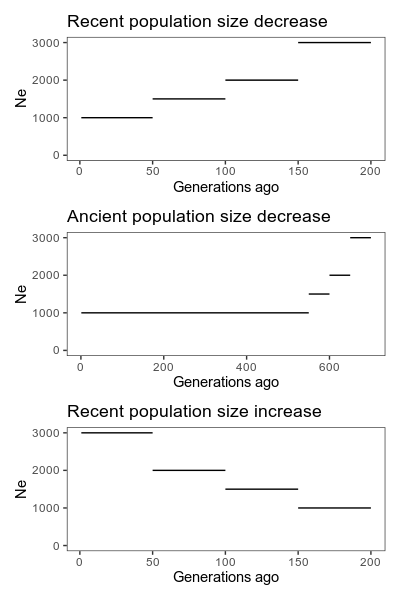
We simulate a constant population, a population that decreased in size relatively recently, a population that increased in size recently, and a population that decreased in longer ago. The latter should be outside of what these methods can comfortably estimate. Finally, let’s also include a population that has migration from an other (unseen) population. Again, that should be a case these methods struggle with.

Simulated true population histories. Note that the horizontal axis is generations ago, meaning that if you read left to right, it runs backwards in time. This is typical when showing population histories like this, but can be confusing. Also not the different scales on the horizontal axis.

library(AlphaSimR)
library(purrr)
library(tibble)

## Population histories

recent_decrease <- tibble(generations = c(1, 50, 100, 150),
                          Ne = c(1000, 1500, 2000, 3000))

recent_increase <- tibble(generations = c(1, 50, 100, 150),
                          Ne = c(3000, 2000, 1500, 1000))

ancient_decrease <- tibble(generations = recent_decrease$generations + 500,
                           Ne = recent_decrease$Ne)

We can feed these population histories (almost) directly into AlphaSimR’s runMacs2 function. The migration case is a little bit more work because we will to modify the command, but AlphaSimR still helps us. MaCS takes a command line written using the same arguments as the paradigmatic ms program. The runMacs2 function we used above generates the MaCS command line for us; we can ask it to just return the command for us to modify. The split argument tells us that we want two populations that split 100 generations ago.

runMacs2(nInd = 100,
         Ne = recent_decrease$Ne[1],
         histGen = recent_decrease$generations[-1],
         histNe = recent_decrease$Ne[-1],
         split = 100,
         returnCommand = TRUE)

The resulting command looks like this:

"1e+08 -t 1e-04 -r 4e-05 -I 2 100 100  -eN 0.0125 1.5 -eN 0.025 2 -eN 0.0375 3 -ej 0.025001 2 1"

The first part is the number of basepairs on the chromosome, -t flag is for the population mutation rate \theta = 4 N_e \mu, -r for the recombination rate (also multiplied by four times the effective population size). The -eN arguments change the population size, and the -ej argument is for splitting and joining populations.

We can check that these numbers make sense: The population mutation rate of 10-4 is the typical per nucleotide mutation rate of 2.5 × 10⁻⁸ multiplied by four times the final population size of 1000. The scaled recombination rate of 4 × 10⁻⁵ is typical per nucleotide recombination rate of 10-8 multiplied by the same.

The population size changes (-eN arguments) are of the format scaled time followed by a scaling of the final population size. Times are scaled by four times the final population size, again. This means that 0.0125 followed by 1.5 refers to that 4 × 0.0125 × 1000 = 50 generations ago population size was 1.5 times the final population size, namely 1500. And so on.

-I (I assume for ”island” as in the ”island model”) sets up the two populations, each with 100 individuals and a migration rate between them. We modify this by setting it to 200 for the first population (because we want diploid individuals, so we need double the number of chromosomes) and 0 for the other; that is, this ghost population will not be observed, only used to influence the first one by migration. Then we set the third parameter, that AlphaSimR has not used: the migration rate. Again, this is expressed as four times the final population size, so for a migration rate of 0.05 we put 200.

Now we can run all cases to generate samples of 100 individuals.

migration_command <- "1e+08 -t 1e-04 -r 4e-05 -I 2 200 0 200  -eN 0.0125 1.5 -eN 0.025 2 -eN 0.0375 3 -ej 0.025001 2 1"

pops <- list(pop_constant = runMacs2(nInd = 100,
                                     nChr = 5,
                                     histNe = NULL,
                                     histGen = NULL,
                                     Ne = 1000),
             
             pop_recent = runMacs2(nInd = 100,
                                   nChr = 5,
                                   Ne = recent_decrease$Ne[1],
                                   histGen = recent_decrease$generations[-1],
                                   histNe = recent_decrease$Ne[-1]),
             
             pop_increase = runMacs2(nInd = 100,
                                     nChr = 5,
                                     Ne = recent_increase$Ne[1],
                                     histGen = recent_increase$generations[-1],
                                     histNe = recent_increase$Ne[-1]),
             
             pop_ancient = runMacs2(nInd = 100,
                                    nChr = 5,
                                    Ne = ancient_decrease$Ne[1],
                                    histGen = ancient_decrease$generations[-1],
                                    histNe = ancient_decrease$Ne[-1]),
             
             pop_migration = runMacs(nInd = 100,
                                     nChr = 5,
                                     manualCommand = migration_command,
                                     manualGenLen = 1))

Both GONE and SNeP work with text files in Plink ped/map format. Look in the repository if you want to see the not too exciting details of how we extract 10 000 markers and save them to Plink format together with their positions.

Running GONE

GONE source code and binaries are found in their GitHub repository, which we can clone or simply download from the web. As I’m running on Linux, we will use the binaries in the Linux subfolder. Before doing anything else, we will have to set the permissions for each of the binaries stored in the PROGRAMMES directory, with chmod u+x to make them executable.

GONE consists of a set of binaries and a bash script that runs them in order. As the as the script assumes it’s always running from the directory where you put GONE and always writes the output files into the same directory, the easiest way to handle it is to duplicate the entire GONE directory for every run. This also duplicates the INPUT_PARAMETERS_FILE file that one would modify to change settings. Then, invoking GONE with default settings would be as simple as opening a terminal, moving to the working directory and running the script, feeding it the base name of the Plink file:

./script_GONE.sh pop_constant

Thus, we write a prep script like this that copies the entire folder, puts the data into it, and then runs GONE:

#!/bin/bash

## Gone needs all the content of the operating system-specific subfolder to be copied
## into a working directory to run from. Therefore we create the "gone" directory
## and copy in the Linux version of the software from the tools directory.

mkdir gone

cd gone

cp -r ../tools/GONE/Linux/* .

## Loop over all the cases and invoke the GONE runscript. Again, because GONE
## needs the data to be in the same directory, we copy the data files into the
## working directory.

for CASE in pop_constant pop_recent pop_ancient pop_migration pop_increase; do

  cp ../simulation/${CASE}.* .
  
  ./script_GONE.sh ${CASE}
  
done

GONE puts its output files (named with the prefixes Output_Ne_, Output_d2_ and OUTPUT_ followed by the base name of the input files) in the same directory. The most interesting is Output_Ne_ which contains the estimates and the all caps OUTPUT_ file that contains logging information about the run.

Estimates look like this:

Ne averages over 40 independent estimates.
Generation      Geometric_mean
1       1616.29
2       1616.29
3       1616.29
4       1616.29
5       1291.22
6       1221.75
7       1194.16
8       1157.95
...

And the log looks like this:

TOTAL NUMBER OF SNPs
10000


HARDY-WEINBERG DEVIATION
-0.009012       Hardy-Weinberg deviation (sample)
-0.003987       Hardy-Weinberg deviation (population)


CHROMOSOME 1
 NIND(real sample)=100
 NSNP=2000
 NSNP_calculations=2000
 NSNP_+2alleles=0
 NSNP_zeroes=0
 NSNP_monomorphic=0
 NIND_corrected=100.000000
 freq_MAF=0.005000
 F_dev_HW (sample)=-0.009017
 F_dev_HW (pop)=-0.003992
 Genetic distances available in map file
...

I will now discuss a couple of issues I ran into. Note, this should not be construed as any kind of criticism of the programs or their authors. Everyone is responsible for their own inability to properly read manuals; I just leave them here in case they are helpful to someone else.

  • If you forget to set the permissions of the binaries, the error message will look like this:/
DIVIDE .ped AND .map FILES IN CHROMOSOMES
./script_GONE.sh: line 96: ./PROGRAMMES/MANAGE_CHROMOSOMES2: Permission denied
RUNNING ANALYSIS OF CHROMOSOMES ...
cp: cannot stat 'chromosome*': No such file or directory
bash: ./PROGRAMMES/LD_SNP_REAL3: Permission denied
...
  • Whereas Plink allows various different kinds of allele symbols in .ped files, GONE does not like allele codes that don’t look like A, C, G or T. The error message for other symbols looks like this:
DIVIDE .ped AND .map FILES IN CHROMOSOMES
RUNNING ANALYSIS OF CHROMOSOMES ...
CHROMOSOME ANALYSES took 0 seconds
Running GONE
 Format error in file outfileLD
 Format error in file outfileLD
 Format error in file outfileLD
 Format error in file outfileLD
 Format error in file outfileLD
...

Running SNeP

SNeP is only available as binaries on its Sourceforge page. Again, I’m using Linux binaries, so I downloaded the Linux binary from there and put it into a tools folder. The binary can be run from any directory, controlling the settings with command line flags. This would run SNeP on one of our simulated datasets, using the Haldane mapping function and correction of linkage disequilibrium values for sample size; these seem to be reasonable defaults:

./SNeP1.1 -ped simulation/pop_constant.ped -out snep/pop_constant -samplesize 2 -haldane

Thus, we write a run script like this:

#!/bin/bash

## As opposed to GONE, SNeP comes as one binary that can run from any directory. We still create
## a working directory to keep the output files in.

mkdir snep

## We loop over all cases, reading the data from the "simulation" directory,
## and directing the output to the "snep" directory. The settings are to
## correct r-squared for sample size using the factor 2, and to use the Haldane
## mapping function. We direct the output to a text file for logging purposes.

for CASE in pop_constant pop_recent pop_ancient pop_migration pop_increase; do

  ./tools/snep/SNeP1.1 \
    -ped simulation/${CASE}.ped \
    -out snep/${CASE} \
    -samplesize 2 \
    -haldane > snep/${CASE}_out.txt
  
done

SNeP creates two ouptut files with the given prefix, one with the extension .NeAll with the estimates a log file with the suffix SNeP.log file. Above, we also save the standard output to another log file.

Estimates look like this:

GenAgo	Ne	dist	r2	r2SD	items
13	593	3750544	0.0165248	0.0241242	37756
15	628	3272690	0.017411	0.0256172	34416
18	661	2843495	0.0184924	0.0281098	30785
20	681	2460406	0.0200596	0.0310288	27618
24	721	2117017	0.0214468	0.0313662	24898
...

Issues I ran into:

  • There are two versions of SNeP on Sourceforge, version 1.1 and version 11.1. According to the readme, SNeP requires ”GCC 4.8.2 or newer”, which I guess is a way to say that it needs a recent enough version of GLIBC, the runtime library that includes the C++ standard library. SNeP 1.11 appears to depend on GLIBC 2.29, and because I have 2.27, I had to use SNeP version 1.1 instead. It might be possible that it doesn’t require the new version of glibc, and that one could build from source on my system — but the source is not available, so who knows; this is a problem with distributing software as binaries only.
  • You cannot specify just a file name for your output. It needs to be a directory followed by a file name; that is, ”snep_constant” is not okay, but ”./snep_constant” is. The error looks like this:
/tools/snep/SNeP1.1 -ped constant.ped -out snep_constant
*************************************
*                SNeP               *
*                v1.1               *
*       barbatom@cardiff.ac.uk      *
*************************************

Sat Dec 25 13:09:38 2021

The -out path provided gives an error, aborting.

The moment you’ve been waiting for

Let’s read the results and look at the estimates!

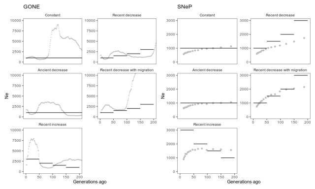
Estimates from GONE, with default settings, and SNeP, with reasonable setting used in the SNeP paper, applied to simulated data from different scenarios. Grey dots are estimates, and black lines the true simulated population history. The estimates go on for a while, but as per the GONE paper’s recommendations, we should not pay attention to estimates further back in time where these methods are not accurate. That is, we should probably concentrate on the first 100 generations or so.

Again, this isn’t a systematic methods evaluation, so this shouldn’t be taken as a criticism of the programs or methods. But we can note that in these circumstances, the estimates capture some features of the simulated population histories but gets other features quite wrong. GONE estimates a recent decrease in the scenario with a recent decrease, but not the further decreases before, and a recent increase when there was a recent increase, but overestimates its size by a few thousand. In the migration scenario, GONE shows the kind of artefact the authors tell us to expect, namely a drastic population size drop. Unexpectedly, though, it estimates a similar drastic drop in the scenario with constant population size. SNeP captures the recent decrease, but underestimates its size. In fact, SNeP estimates a similar shape in all scenarios, both for increased, decreased and constant populations.

The plotting code looks something like this (see GitHub for the details): we create the file names, read all the output files into the same data frame with map_dfr, label them by what case they belong to by joining with the data frame of labels (with inner_join from dplyr) and make a plot with ggplot2. The true_descriptions data frame contains the true population histories used to simulate the data.

library(ggplot2)
library(readr)

cases <- tibble(case = c("pop_constant",
                         "pop_recent",
                         "pop_ancient",
                         "pop_migration",
                         "pop_increase"),
                description = c("Constant",
                                "Recent decrease",
                                "Ancient decrease",
                                "Recent decrease with migration",
                                "Recent increase"))

snep_file_names <- paste("snep/", cases$case, ".NeAll", sep = "")
names(snep_file_names) <- cases$case

snep <- map_dfr(snep_file_names, read_tsv, .id = "case")


snep_descriptions <- inner_join(snep, cases)
snep_descriptions$description <- factor(snep_descriptions$description,
                                        levels = cases$description)

## Make both a plot of the entire range of estimates, and a plot of the
## first 200 generations, which is the region where estimates are expected
## to be of higher quality
plot_snep_unconstrained <- ggplot() +
  geom_point(aes(x = GenAgo, y = Ne),
             data = snep_descriptions,
             colour = "grey") +
  facet_wrap(~ description,
             scale = "free_y",
             ncol = 2) +
  geom_segment(aes(x = start,
                   y = Ne,
                   xend = end,
                   yend = Ne),
               data = true_descriptions) +
  theme_bw() +
  theme(panel.grid = element_blank(),
        strip.background = element_blank()) +
  xlab("Generations ago")

plot_snep <- plot_snep_unconstrained +
  coord_cartesian(xlim = c(0, 200), ylim = c(0, 3000))

När kartan inte stämmer med terrängen gäller terrängen

When the results of a method don’t agree with the parameters of simulated data, the problem can either lie with the method or with the simulated data. And in this case, coalescent simulation is known to have problems with linkage disequilibrium. Here is a figure (Fig A, of appendix 2) of Nelson et al. (2020) who study the problems with coalescent simulations over long regions (such as the ones we simulated here).

The problem occurs for variants that are far apart (e.g. at around 100 = 1 expected recombinations between loci), where there should still be linkage disequilibrium, whereas the coalescent simulator (in this figure, ”msprime (Hudson)”) gives too low linkage disequilibrium. When we try to estimate effective population size late in population history, the methods rely on linkage equilibrium between markers far apart, and if they have too low linkage disequilibrium, the estimated population size should be too large. This does not appear to be what is going on here, but there might be more subtle problems with the simulated linkage disequilibrium that fools these methods; we could try something like Nelson et al.’s hybrid method or a forward simulation instead.

Literature

Barbato, M., Orozco-terWengel, P., Tapio, M., & Bruford, M. W. (2015). SNeP: a tool to estimate trends in recent effective population size trajectories using genome-wide SNP data. Frontiers in genetics, 6, 109.

Nelson, D., Kelleher, J., Ragsdale, A. P., Moreau, C., McVean, G., & Gravel, S. (2020). Accounting for long-range correlations in genome-wide simulations of large cohorts. PLoS genetics, 16(5), e1008619.

Santiago, E., Novo, I., Pardiñas, A. F., Saura, M., Wang, J., & Caballero, A. (2020). Recent demographic history inferred by high-resolution analysis of linkage disequilibrium. Molecular Biology and Evolution, 37(12), 3642-3653.

Journal club of one: ”A unifying concept of animal breeding programmes”

The developers of the MoBPS breeding programme simulators have published three papers about it over the last years: one about the MoBPS R package (Pook et al. 2020), one about their web server MoBPSweb (Pook et al. 2021), and one that discusses the logic of the specification for breeding programmes they use in the web interface (Simianer et al. 2021). The idea is that this specification can be used to describe breeding programmes in a precise and interoperable manner. The latter — about breeding programme specification — reads as if the authors had a jolly good time thinking about what breeding and breeding programmes are; at least, I had such feelings while reading it. It is accompanied by an editorial by Simianer (2021) talking about what he thinks are the important research directions for animal breeding research. Using simulation to aid breeding programme design is one of them.

Defining and specifying breeding programmes

After defining a breeding programme in a narrow genetic sense as a process achieving genetic change (more about that later), Simianer et al. (2021) go on to define a specification of such a breeding programme — or more precisely, of a model of a breeding programme. They use the word ”definition” for both things, but they really talk about two different things: defining what ”a breeding programme” is and specifying a particular model of a particular breeding programme.

Here, I think it is helpful to think of Guest & Martin’s (2020) distinction, borrowed from psychology, between a specification of a model and an implementation of a model. A specification is a description of a model based in natural language or math. Breeding programme modelling often takes the shape of software packages, where the software implementation is the model and a specification is quite vague. Simianer et al. (2021) can be seen as a step towards a way of writing specifications, on a higher level in Guest & Martin’s hierarchy, of what such a breeding programme model should achieve.

They argue that such a specification (”formal description”) needs to be comprehensive, unambiguous and reproducible. They claim that this can be achieved with two parts: the breeding environment and the breeding structure.

The breeding environment includes:

  • founder populations,
  • quantitative genetic parameters for traits,
  • genetic architectures for traits,
  • economic values for traits in breeding goal,
  • description of genomic information,
  • description of breeding value estimation methods.

Thus, the ”formal” specification depends on a lot of information that is either unknowable in practice (genetic architecture), estimated with error (genetic parameters), hard to describe other than qualitatively (founder population) and dependent on particular software implementations and procedures (breeding value estimation). This illustrates the need to distinguish the map from the territory — to the extent that the specification is exact, it describes a model of a breeding programme, not a real breeding programme.

The other part of their specification is the graph-based model of breeding structure. I think this is their key new idea. The breeding structure, in their specification, consists of nodes that represent groups of elementary objects (I would say ”populations”) and edges that represent transformations that create new populations (such as selection or mating) or are a shorthand for repeating groups of edges and nodes.

The elementary objects could be individuals, but they also give the example of gametes and genes (I presume they mean in the sense of alleles) as possible elementary objects. One could also imagine groups of genetically identical individuals (”genotypes” in a plant breeding sense). Nodes contain a given number of individuals, and can also have a duration.

Edges are directed, and correspond to processes such as ageing, selection, reproduction, splitting or merging populations. They will carry attributes related to the transformation. Edges can have a time associated with them that it takes for the transformation to happen (e.g. for animals to gestate or grow to a particular age). Here is an example from Pook et al. (2021) of a breeding structure graph for dairy cattle:

If we ignore the red edges for now, we can follow the flow of reproduction (yellow edges) and selection (green edges): The part on the left is what is going on in the breeding company: cows (BC-Cows) reproduce with selected bulls (BC-SelectedBulls), and their offspring become the next generation of breeding company cows and bulls (BC-NextCows and BC-NextBulls). On the right is the operation of a farm, where semen from the breeding company is used to inseminate cows and heifers (heifer, cow-L1, cow-L2, cow-L3) to produce calfs (calf-h, calf-L1, calf-L2, calf-L3). Each cycle each of these groups, through a selection operation, give rise to the next group (heifers becoming cows, first lactation cows becoming second lactation cows etc).

Breeding loops vs breeding graphs vs breeding forms

Except for the edges that specify breeding operations, there is also a special meta-edge type, the repeat edge, that is used to simplify breeding graphs with repeated operations.

A useful edge class to describe breeding programmes that are composed of several breeding cycles is ”repeat.” It can be used to copy resulting nodes from one breeding cycle into the nodes of origin of the next cycle, assuming that exactly the same breeding activities are to be repeated in each cycle. The “repeat” edge has the attribute “number of repeats” which allows to determine the desired number of cycles.

In the MoBPSweb paper (Pook et al. 2020), they describe how it is implemented in MoBPS: Given a breeding specification in MoBPSweb JSON format, the simulator will generate a directed graph by copying the nodes on the breeding cycle as many times as is specified by the repeat number. In this way, repeat edges are eliminated to make the breeding graph acyclic.

The conversion of the breeding scheme itself is done by first detecting if the breeding scheme has any “Repeat” edges (Simianer et al. 2020), which are used to indicate that a given part of the breeding programme is carried out multiple times (breeding cycles). If that is the case, it will subsequently check which nodes can be generated without the use of any repeat. Next, all repeats that can be executed based on the already available nodes are executed by generating copies of all nodes between the node of origin and the target node of the repeat (including the node of origin and excluding the target node). Nodes generated via repeat are serial-numbered via “_1,” “_2” etc. to indicate the repeat number. This procedure is repeated until all repeat edges are resolved, leading to a breeding programme without any repeats remaining.

There are at least three ways to specify the breeding structures for breeding programme simulations: these breeding graphs, breeding loops (or more generally, specifying breeding in a programming language) and breeding forms (when you get a pre-defined breeding structure and are allowed fill in the numbers).

If I’m going to compare the graph specification to what I’m more familiar with, this is how you would create a breeding structure in AlphaSimR:

library(AlphaSimR)

## Breeding environment

founderpop <- runMacs(nInd = 100,
                      nChr = 20)
simparam <- SimParam$new(founderpop)
simparam$setSexes("yes_sys")
simparam$addTraitA(nQtlPerChr = 100)
simparam$setVarE(h2 = 0.3)

## Breeding structure

n_time_steps <- 10

populations <- vector(mode = "list",
                      length = n_time_steps + 1)

populations[[1]] <- newPop(founderpop,
                           simParam = simparam)

for (gen_ix in 2:(n_time_steps + 1)) {

  ## Breeding cycle happens here

}

In the AlphaSimR script, the action typically happens within the loop. You apply different functions on population objects to make your selection, move individuals between parts of the breeding programme, create offspring etc. That is, in the MoBPS breeding structure, populations are nodes and actions are edges. In AlphaSimR, populations are objects and operations are functions. In order to not have to copy paste your breeding code, you use the control flow structures of R to make a loop (or some functional equivalent). In MoBPS graph structure, in order to not have to create every node and edge manually, you use the Repeat edge.

Breeding graphs with many repeat edges with different times attached to them have the potential to be complicated, and the same is true of breeding loops. I would have to use both of them more to have an opinion about what is more or less intuitive.

Now that we’ve described what they do in the paper, let’s look at some complications.

Formal specifications only apply to idealised breeding programmes

The authors claim that their concept provides a formal breeding programme specification (in their words, ”formal description”) that can be fully understood and implemented by breeders. It seems like the specification fails to live up to this ambition, and it appears doubtful whether any type of specification can. This is because they do not distinguish between specifying a model of a breeding programme and specifying a real implementation of a breeding programme.

First, as mentioned above, the ”breeding environment” as described by them, contains information that can never be specified for any real population, such as the genetic architecture of complex traits.

Second, their breeding structure is described in terms of fixed numbers, which will never be precise due to mortality, conception rates, logistics and practical concerns. They note such fluctuations in population size as a limitation in the Discussion. To some extent, random mortality, reproductive success etc an be modelled by putting random distributions on various parameters. (I am not sure how easy this is to do in the MoBPS framework; it is certainly possible.) However, this adds uncertainty about what these hyperparameter should be and whether they are realistic.

Such complications would just be nit-picking if the authors had not suggested that their specification can be used to communicate breeding programmes between breeders and between breeders and authorities, such as when a breeding programme is seeking approval. They acknowledge that the authorities, for example in the EU, want more detailed information that are beyond the scope of their specification.

And the concept is not very formal in the first place

Despite the claimed formality, every class of object in the breeding structure is left open, with many possible actions and many possible attributes that are never fully defined.

It is somewhat ambiguous what is to be the ”formal” specification — it cannot be the description in the paper as it is not very formal or complete; it shouldn’t be the implementation in MoBPS and MoBPSweb, as the concept is claimed to be universal; maybe it is the JSON specification of the breeding structure and background as described in the MoBPSweb paper (Pook et al. 2020). The latter seems the best candidate for a well-defined formal way to specify breeding programme models, but then again, the JSON format appears not to have a published specification, and appears to contain implementation-specific details relating to MoBPS.

This also matters to the suggested use of the specification to communicate real breeding programme designs. What, precisely, is it that will be communicated? Are breed societies and authorities expected to communicate with breeding graphs, JSON files, or with verbal descriptions using their terms (e.g. ”breeding environment”, ”breeding structure”, their node names and parameters for breeding activities)?

There is almost never a need for a definition

As I mentioned before, the paper starts by asking what a breeding programme is. They refer to different descriptions of breeding programme design from textbooks, and a legal definition from EU regulation 2016/1012; article 2, paragraph 26, which goes:

‘breeding programme’ means a set of systematic actions, including recording, selection, breeding and exchange of breeding animals and their germinal products, designed and implemented to preserve or enhance desired phenotypic and/or genotypic characteristics in the target breeding population.

There seems to be some agreement that a breeding programme, in addition to being the management of reproduction of a domestic animal population, also is systematic and goal-directed activity. Despite these descriptions of breeding programmes and their shared similarity, the authors argue that there is no clear formal definition of what a breeding programme is, and that this would be useful to delineate and specify breeding programmes.

They define a breeding programme as an organised process that aims to change the genetic composition in a desired direction, from one group of individuals to a group of individuals at a later time. The breeding programme comprises those individuals and activities that contribute to this process. For example, crossbred individuals in a multiplier part of a terminal crossbreeding programme would be included to the extent that they contribute information to the breeding of nucleus animals.

We define a breeding programme as a structured, man-driven process in time that starts with a group of individuals X at time t_1 and leads to a group of individuals Y at time t_2 > t_1. The objective of a breeding programme is to transform the genetic characteristics of group X to group Y in a desired direction, and a breeding programme is characterized by the fact that the implemented actions aim at achieving this transformation.

They actually do not elaborate on what it means that a genetic change has direction, but since they want the definition to apply both to farm animal and conservation breeding programmes, the genetic goals could be formulated both in terms of changes in genetic values for traits and in terms of genetic relationships.

Under many circumstances, this is a reasonable proxy also for an economic target: The breeding structures and interventions considered in theoretical breeding programme designs can often be evaluated in terms of their effect on the response to selection, and if the response improves, so will the economic benefit. However, this definition seems a little unnecessary and narrow. If you wanted to, say, add a terminal crossbreeding step to the simulation and evaluate the performance in terms of the total profitability of the crossbreeding programme (that is, something that is outside of the breeding programme in the sense of the above definition), nothing is stopping you, and the idea is not in principle outside of the scope of animal breeding.

Finally, an interesting remark about efficiency

When discussing the possibility of using their concept to communicate breeding programmes to authorities when seeking approval the authors argue that authorities should not take efficiency of the breeding programme into account when they evaluate breeding programmes for approval. They state this point forcefully without explaining their reasoning:

It should be noted, though, that an evaluation of the efficiency of breeding programme is not, and should never be, a precondition for the approval of a breeding programme by the authorities.

This raises the question: why not? There might be both environmental, economical and animal ethical reasons to consider not approving breeding programmes that can be shown to make inefficient use of resources. Maybe such evaluation would be impractical — breeding programme analysis and simulation might have to be put on a firmer scientific grounding and be made more reproducible and transparent before we trust it to make such decisions — but efficiency does seem like an appropriate thing to want in a breeding scheme, also from the perspective of society and the authorities.

I am not advocating any particular new regulation for breeding programmes here, but I wonder where the ”should never” came from. This reads like a comment added to appease a reviewer — the passage is missing from the preprint version.

Literature

Pook, T., Schlather, M., & Simianer, H. (2020a). MoBPS-modular breeding program simulator. G3: Genes, Genomes, Genetics, 10(6), 1915-1918. https://academic.oup.com/g3journal/article/10/6/1915/6026363

Pook, T., Büttgen, L., Ganesan, A., Ha, N. T., & Simianer, H. (2021). MoBPSweb: A web-based framework to simulate and compare breeding programs. G3, 11(2), jkab023. https://academic.oup.com/g3journal/article/11/2/jkab023/6128572

Simianer, H., Büttgen, L., Ganesan, A., Ha, N. T., & Pook, T. (2021). A unifying concept of animal breeding programmes. Journal of Animal Breeding and Genetics, 138 (2), 137-150. https://onlinelibrary.wiley.com/doi/full/10.1111/jbg.12534

Simianer, H. (2021), Harvest Moon: Some personal thoughts on past and future directions in animal breeding research. J Anim Breed Genet, 138: 135-136. https://doi.org/10.1111/jbg.12538

Guest, O., & Martin, A. E. (2020). How computational modeling can force theory building in psychological science. Perspectives on Psychological Science, 1745691620970585. https://journals.sagepub.com/doi/full/10.1177/1745691620970585

Journal club of one: ”Versatile simulations of admixture and accurate local ancestry inference with mixnmatch and ancestryinfer”

Admixture is the future of every sub-field of genetics, just in case you didn’t know. Both in the wild and domestic animals, populations or even species sometimes cross. This causes different patterns of relatedness than in well-mixed populations. Often we want to estimate ”local ancestry”, that is: what source population a piece of chromosome in an individual originates from. It is one of those genetics problems that is made harder by the absence of any way to observe it directly.

This recent paper (Schumer et al 2020; preprint version, which I read, here) presents a method for simulating admixed sequence data, and a method for inferring local ancestry from it. It does something I like, namely to pair analysis with fake-data simulation to check methods.

The simulation method is a built from four different simulators:

1. macs (Chen, Majoram & Wall 2009), which creates polymorphism data under neutral evolution from a given population history. They use macs to generate starting chromosomes from two ancestral populations.

2. Seq-Gen (Rambaut & Grassly 1997). Chromosomes from macs are strings of 0s and 1s representing the state at biallelic markers. If you want DNA-level realism, with base composition, nucleotide substitution models and so on, you need something else. I don’t really follow how they do this. You can tell from the source code that they use the local trees that macs spits out, which Seq-Gen can then simulate nucleotides from. As they put it, the resulting sequence ”lacks other complexities of real genome sequences such as repetitive elements and local variation in base composition”, but it is a step up from ”0000110100”.

3. SELAM (Corbett-Detig & Jones 2016), which simulates admixture between populations with population history and possibly selection. Here, SELAM‘s role is to simulate the actual recombination and interbreeding to create the patterns of local ancestry, that they will then fill with the sequences they generated before.

4. wgsim, which simulates short reads from a sequence. At this point, mixnmatch has turned a set of population genetic parameters into fasta files. That is pretty cool.

On the one hand, building on tried and true tools seems to be the right thing to do, less wheel-reinventing. It’s great that the phylogenetic simulator Seq-Gen from 1997 can be used in a paper published in 2020. On the other hand, looking at the dependencies for running mixnmatch made me a little pale: seven different bioinformatics or population genetics softwares (not including the dependencies you need to compile them), R, Perl and Python plus Biopython. Computational genetics is an adventure of software installation.

They use the simulator to test the performance of a hidden Markov model for inferring local ancestry (Corbett-Detig & Nielsen 2017) with different population histories and settings, and then apply it to swordtail fish data. In particular, one needs to set thresholds for picking ”ancestry informative” (i.e. sufficiently differentiated) markers between the ancestral populations, and that depends on population history and diversity.

In passing, they use the estimate the swordtail recombination landscape:

We used the locations of observed ancestry transitions in 139 F2 hybrids that we generated between X. birchmanni and X. malinche … to estimate the recombination rate in 5 Mb windows. … We compared inferred recombination rates in this F2 map to a linkage disequilibrium based recombination map for X. birchmanni that we had previously generated (Schumer et al., 2018). As expected, we observed a strong correlation in estimated recombination rate between the linkage disequilibrium based and crossover maps (R=0.82, Figure 4, Supporting Information 8). Simulations suggest that the observed correlation is consistent with the two recombination maps being indistinguishable, given the low resolution of the F2 map (Supporting Information 8).

Paper: ‘Removal of alleles by genome editing (RAGE) against deleterious load’

Our new paper is about using predicted deleterious variants in animal breeding. We use simulation to look at the potential to improve livestock fitness by either selecting on detected deleterious variants or removing deleterious alleles by genome editing.

Summary

Deleterious variants occur when errors in DNA replication that disrupt the function of a gene. Such errors are frequent enough that all organisms carry mildly deleterious variants. Geneticists describe this as a deleterious load, that cause organisms to be less healthy and fit than they could have been if these errors didn’t happen. Load is especially pertinent to livestock populations, because of their relatively small population sizes and inbreeding.

Historically, it has not been possible to observe deleterious variants directly, but as genome sequencing becomes cheaper and new bioinformatic methods are being developed, we can now sequence livestock and detect variants that are likely to be deleterious.

In this study, we used computer simulation to see how future breeding strategies involving selection or genome editing could be used to reduce deleterious load. We tested selection against deleterious load and genome editing strategy we call RAGE (Removal of Alleles by Genome Editing) in simulated livestock populations to see how it improved fitness. The simulations suggest that selecting on deleterious variants identified from genome sequencing may help improve fitness of livestock populations, and that genome editing to remove deleterious variants could improve them even more.

For these strategies to be effective, it is important that detection of deleterious variants is accurate, and genome editing of more than one variant per animal would need to become possible without damaging side-effects. Future research on how to measure deleterious load in large sequence datasets from livestock animals, and how to perform genome editing safely and effectively will be important.

Figure 2 from the paper, showing the average fitness of simulated populations (y-axis) over the generations of breeding (x-axis) with different types of future breeding against deleterious variants.

‘RAGE against …’, what’s with the acronym?

We are very happy with the acronym. In addition to making at least two pop culture references, it’s also a nod to Promotion of Alleles by Genome Editing (PAGE) from Jenko et al. (2015). I like that the acronyms, both PAGE and RAGE, emphasises that we’re dealing with alleles that already exist within a population. We propose using genome editing as a way to promote alleles we like and remove alleles we don’t like in addition to classical breeding. The fancy new biotechnology does not replace selection, but supplements it.

Do you really think one should genome edit farm animals?

Yes, if all the bio- and reproductive technology can be made to work! Currently, genome editing methods like Crispr/Cas9 require many attempts to get precise editing to the desired allele at one place, and it doesn’t scale to multiple edits in the same animal … Not yet. But lots of smart people are competing to make it happen.

Genome editing of farm animals would also need a lot of reproductive technology, that currently isn’t really there (but probably more so for cattle than for other species). Again, lots of clever people work on it.

If it can be made to work, genome editing could be a useful breeding method.

What about the ethics of genome editing?

We don’t discuss ethics much in the paper. In one simple sense, that is because ethics isn’t our expertise. I also think a discussion of the ethics of RAGE, much like an informed discussion about the economics of it, requires empirical knowledge that we don’t have yet.

I am not of the opinion that there is a dignity or integrity to the genome that would prohibit genome editing as a rule. So the question is not ‘genome editing or not’, but ‘under what circumstances and for what applications is genome editing useful and justified?’ and ‘are the benefits of RAGE, PAGE, or whatever -GE, enough to outweigh the risks and costs?’. There is room for uncertainty and disagreement about those questions.

For a good discussion of the ethics of genome editing that is likely to raise more questions than it answers, see Eriksson et al. (2018). Among other things, they make the point that advanced reproductive technologies is a precondition for genome editing, but kind of slips out of the discussion sometimes. I think the most pressing question, both from the ethical and economical perspective, is whether the benefits of genome editing are enough to justify widespread use of reproductive technologies (in species where that isn’t already commonplace). I also like how they make the point that one needs to look at the specific applications of genome editing, in context, when evaluating them.

The simulation looks nifty! I want to simulate breeding programs like that!

You can! The simulations used the quantitative genetic simulation R package AlphaSimR with some modifications for simulating the fitness traits. There is code with the paper. Here are also the slides from when I talked about the paper at the Edinburgh R user group.

You make a ton of assumptions!

We do. Some of them are extremely uncontroversial (the basic framework of segregation and recombination during inheritance), some we can get some idea about by looking at the population genetics literature (we’ve taken inspiration from estimates of deleterious mutation rates and effect distributions estimated from humans), and some we don’t have much knowledge about at all (how does load of deleterious variants relate to the production, reproduction and health traits that are important to breeding? The only way to know is to measure). If you read the paper, don’t skip that part of the Discussion.

Would this work in plants?

Yes, probably! Plant breeding programs are a bit different, so I guess one should simulate them to really know. RAGE would be a part of the ‘Breeding 4.0’ logic of Wallace, Rodgers-Melnick & Butler (2018). In many ways the problems with plants are smaller, with less unknown reproductive technology that needs to be invented first, and an easier time field testing edited individuals.

Literature

Johnsson M, Gaynor RC, Jenko J, Gorjanc G, de Koning D-J, Hickey, JM. (2019) Removal of alleles by genome editing (RAGE) against deleterious load. Genetics Selection Evolution.

Jenko J, Gorjanc G, Cleveland MA, Varshney RK, Whitelaw CBA, Woolliams JA, Hickey JM. (2015). Potential of promotion of alleles by genome editing to improve quantitative traits in livestock breeding programs. Genetics Selection Evolution.

Eriksson, S., Jonas, E., Rydhmer, L., & Röcklinsberg, H. (2018). Invited review: Breeding and ethical perspectives on genetically modified and genome edited cattle. Journal of dairy science, 101(1), 1-17.

Wallace, J. G., Rodgers-Melnick, E., & Buckler, E. S. (2018). On the road to Breeding 4.0: unraveling the good, the bad, and the boring of crop quantitative genomics. Annual review of genetics, 52, 421-444.

A slightly different introduction to R, part V: plotting and simulating linear models

In the last episode (which was quite some time ago) we looked into comparisons of means with linear models. This time, let’s visualise some linear models with ggplot2, and practice another useful R skill, namely how to simulate data from known models. While doing this, we’ll learn some more about the layered structure of a ggplot2 plot, and some useful thing about the lm function.

11. Using points, lines and error bars to show predictions from linear models

Return to the model of comb gnome mass at time zero. We’ve already plotted the coefficient estimates, but let us just look at them with the coef() function. Here the intercept term is the mean for green comb gnomes subjected to the control treatment. The ‘grouppink’ and ‘treatmentpixies’ coefficients are the mean differences of pink comb gnomes and comb gnomes exposed to pixies from this baseline condition. This way of assigning coefficients is called dummy coding and is the default in R.

model <- lm(mass0 ~ group + treatment, data)
coef(model)[1]
    (Intercept)       grouppink treatmentpixies 
      141.56771       -49.75414        23.52428

The estimate for a pink comb gnome with pixies is:

coef(model)[1] + coef(model)[2] + coef(model)[3]

There are alternative codings (”contrasts”) that you can use. A common one in Anova is to use the intercept as the grand mean and the coefficients as deviations from the mean. (So that the coefficients for different levels of the same factor sum to zero.) We can get this setting in R by changing the contrasts option, and then rerun the model. However, whether the coefficients are easily interpretable or not, they still lead to the same means, and we can always calculate the values of the combinations of levels that interest us.

Instead of typing in the formulas ourself as above, we can get predictions from the model with the predict( ) function. We need a data frame of the new values to predict, which in this case means one row for each combination of the levels of group and treatment. Since we have too levels each there are only for of them, but in general we can use the expand.grid( ) function to generate all possible factor levels. We’ll then get the predictions and their confidence intervals, and bundle everything together to one handy data frame.

levels <- expand.grid(group=c("green", "pink"), treatment=c("control", "pixies"))
predictions <- predict(model, levels, interval="confidence")
predicted.data <- cbind(levels, predictions)
  group treatment       fit       lwr      upr
1 green   control 141.56771 125.82527 157.3101
2  pink   control  91.81357  76.48329 107.1439
3 green    pixies 165.09199 149.34955 180.8344
4  pink    pixies 115.33785  98.93425 131.7414

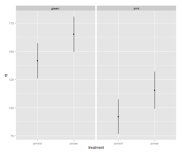
Now that we have these intervals in a data frame we can plot them just like we would any other values. Back in part II, we put several categorical variables into the same plot by colouring the points. Now, let’s introduce nice feature of ggplot2: making small multiples with faceting. qplot( ) takes facets argument which is a formula where the left hand side, before the tilde (‘~’), will be used to split the plot vertically, and the right hand side will split the plot horizontally. In this case, we split horizontally, each panel representing one level of the treatment variable. Also, we use a new geometry: pointrange, which draws a point with bars above and below it and is quite suitable for the intervals we’ve got.

qplot(x=treatment, facets=~group,
      y=fit, ymax=upr, ymin=lwr
      geom="pointrange", data=predicted.data)

model_lineranges

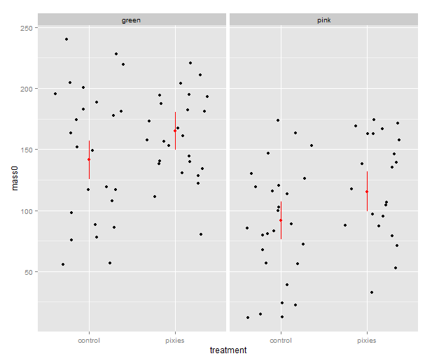
That’s good, but combining the predictions from the model and the actual data in the same plot would be nice. In ggplot2, every plot is an object that can be saved away to a variable. Then we can use the addition operator to add layers to the plot. Let’s make a jittered dotplot like the above and then add a layer with the pointrange geometry displaying confidence intervals. The scatter of the data points around the confidence intervals reminds us that there is quite a bit of residual variance. The coefficient of determination, as seen in the summary earlier, was about 0.25.

qplot(x=treatment, y=mass0, facets=~group, geom="jitter", data=data) +
    geom_pointrange(aes(y=fit, ymax=upr, ymin=lwr), colour="red", data=predicted.data)

model_jitter

In the above, we make use of ggplot2’s more advanced syntax for specifying plots. The addition operator adds layers. The first layer can be set up with qplot(), but the following layers are made with their respective functions. Mapping from variables to features of the plot, called aesthetics, have to be put inside the aes() function. This might look a bit weird in the beginning, but it has its internal logic — all this is described in Hadley Wickham’s ggplot2 book.

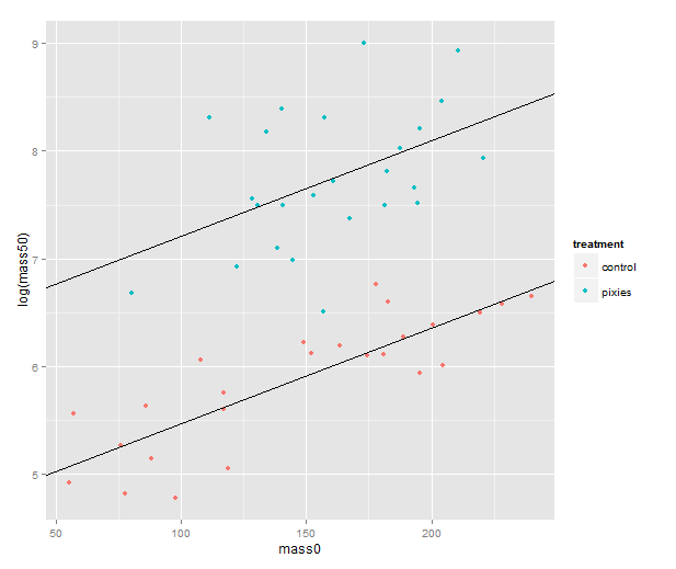
We should probably try a regression line as well. The abline geometry allows us to plot a line with given intercept and slope, i.e. the coefficients of a simple regression. Let us simplify a little and look at the mass at time zero and the log-transformed mass at time 50 in only the green group. We make a linear model that uses the same slope for both treatments and a treatment-specific intercept. (Exercise for the reader: look at the coefficients with coef( ) and verify that I’ve pulled out the intercepts and slope correctly.) Finally, we plot the points with qplot and add the lines one layer at the time.

green.data <- subset(data, group=="green")
model.green <- lm(log(mass50) ~ mass0 + treatment, green.data)
intercept.control <- coef(model.green)[1]
intercept.pixies <- coef(model.green)[1]+coef(model.green)[3]
qplot(x=mass0, y=log(mass50), colour=treatment, data=green.data) +
   geom_abline(intercept=intercept.pixies, slope=coef(model.green)[2]) +
   geom_abline(intercept=intercept.control, slope=coef(model.green)[2])

regression_lines

12. Using pseudorandom numbers for sanity checking

There is a short step from playing with regression functions that we’ve fitted, like we did above, to making up hypothetical regression functions and simulating data from them. This type of fake-data simulation is very useful to for testing how designs and estimation procedures behave and check things like the control of false positive rate and the power to accurately estimate a known model.

The model will be the simplest possible: a single categorical predictor with only two levels and normally distributed equal error variance, i.e. a t-test. There is a formula for the power of the t-test and an R function, power.t.test( ), that calculates it for us without the need for simulation. However, a nice thing about R is that we can pretty easily replace the t-test with more complex procedures. Any model fitting process that you can program in R can be bundled into a function and applied to pseudorandom simulated data. In the next episode we will go into how to make functions and apply them repeatedly.

Let us start out with a no effect model: 50 observations in two groups drawn from the same distribution. We use the mean and variance of the green control group. This first part just sets up the variables:

mu <- mean(subset(data, group=="green" & treatment=="control")$mass0)
sigma <- sd(subset(data, group=="green" & treatment=="control")$mass0)
treatment <- c(rep(1, 50), rep(0, 50))

The rnorm( ) function generates numbers from a normal distribution with specified mean and standard deviation. Apart from drawing numbers from it, R can of course pull out various table values, and it knows other distributions as well. Look at the documentation in ?distributions. Finally we perform a t-test. Most of the time, it should not show a significant effect, but sometimes it will.

sim.null <- rnorm(100, mu, sigma)
t.test(sim.null ~ treatment)$p.value

We can use the replicate( ) function to evaluate an expression multiple times. We put the simulation and t-test together into one expression, rinse and repeat. Finally, we check how many of the 1000 replicates gave a p-value below 0.05. Of course, it will be approximately 5% of them.

sim.p <- replicate(1000, t.test(rnorm(100, mu, sigma) ~ treatment)$p.value)
length(which(sim.p < 0.05))/1000
[1] 0.047

Let us add an effect! Say we’re interested in an effect that we expect to be approximately half the difference between the green and pink comb gnomes:

d <- mean(subset(data, group=="green" & treatment=="control")$mass0) -
     mean(subset(data, group=="pink" & treatment=="control")$mass0)
sim.p.effect <- replicate(1000, t.test(treatment * d/2 +
                                       rnorm(100, mu, sigma) ~ treatment)$p.value)
length(which(sim.p.effect < 0.05))/1000
[1] 0.737

We see that with 50 individuals in each group and this effect size we will detect a significant difference about 75% of the time. This is the power of the test. If you are able to find nice and trustworthy prior information about the kind of effect sizes and variances you expect to find in a study, design analysis allows you to calculate for instance how big a sample you need to have good power. Simulation can also give you an idea of how badly a statistical procedure will break if the assumptions don’t hold. We can try to simulate a situation where the variances of the two groups differs quite a bit.

sim.unequal <- replicate(1000, t.test(c(rnorm(50, mu, sigma),
                                        rnorm(50, mu, 2*sigma)) ~ treatment)$p.value)
length(which(sim.unequal < 0.05))/1000
[1] 0.043
sim.unequal.effect <- replicate(1000, t.test(c(rnorm(50, mu+d/2, sigma),
                                               rnorm(50, mu, 2*sigma)) ~ treatment)$p.value)
length(which(sim.unequal.effect < 0.05))/1000
[1] 0.373

In conclusion, the significance is still under control, but the power has dropped to about 40%. I hope that has given a small taste of how simulation can help with figuring out what is going on in our favourite statistical procedures. Have fun!